The problem
Multi-view depth estimation combines images taken from different viewpoints to recover metric scene geometry. Matching becomes unreliable when views disagree, while strong monocular features do not necessarily preserve the geometry needed for depth reconstruction.
How GeoFusion works
- Geometric Consensus-aware Cost Aggregation (GC-CA) checks whether depth hypotheses agree across views. It suppresses inconsistent evidence before cost aggregation, helping the model avoid misleading matches.
- Geometrically Anchored Feature Rectification (GAFR-Net) uses the multi-view cost volume as a metric anchor to rectify monocular features. This brings learned visual cues into closer agreement with the geometric reconstruction.
- The two components connect reliable multi-view matching with geometry-aware feature fusion, rather than treating matching and feature quality as independent problems.
Inside the architecture
From camera views to a consensus-aware cost volume
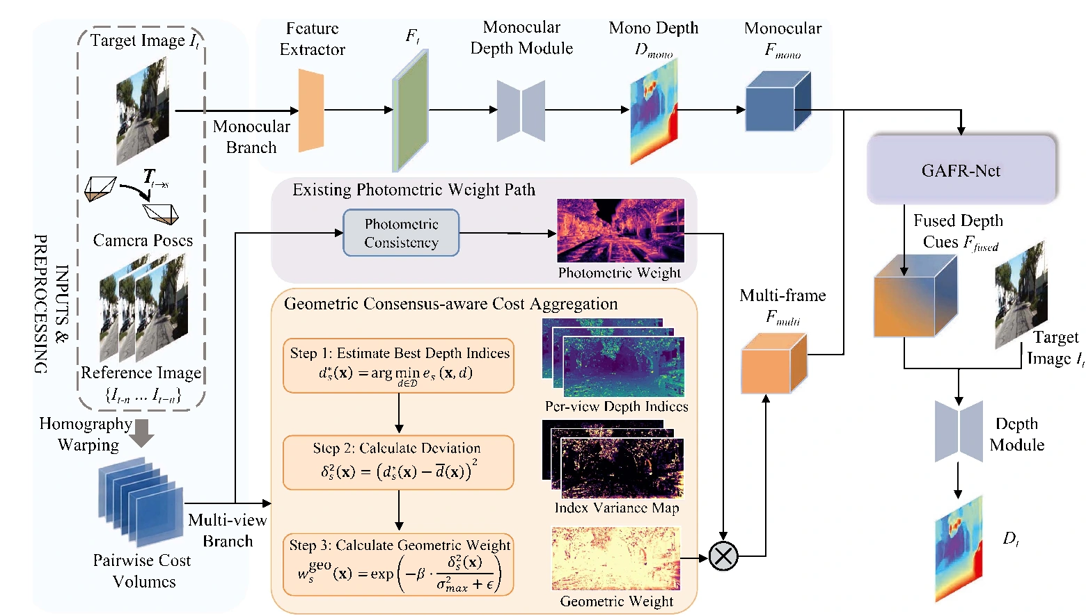
GeoFusion starts from a target image and reference views with camera calibration and relative poses. Reference features are warped into the target camera frustum over inverse-depth hypotheses. These pairwise matches provide the evidence used to estimate depth.
Photometric confidence alone can be misleading in textureless areas, shadows, or occluded regions. GC-CA therefore measures how far each view’s local depth hypothesis deviates from the global consensus. A soft geometric weight suppresses outliers without imposing a hard accept/reject boundary. Multiplying the photometric and geometric weights gives the final view weight used for cost aggregation.
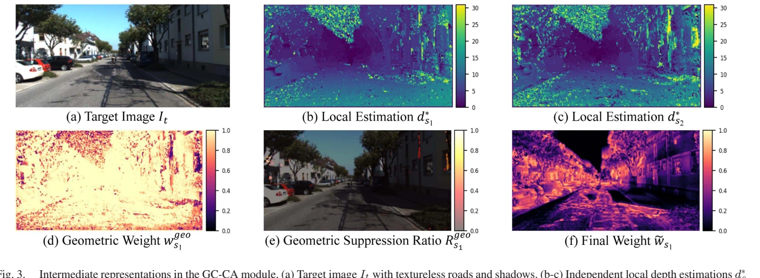
The intermediate maps distinguish photometric confidence from geometric agreement. The suppression map highlights locations where an apparently confident image match lacks support from the other views; the final weight combines both sources of evidence.
Why the fusion has a direction
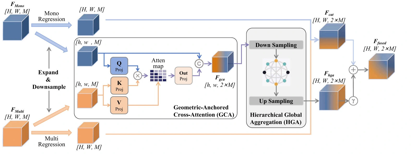
The monocular branch predicts an initial depth map, which is encoded over the same depth hypotheses as the multi-view cost volume. Both representations are embedded before fusion. In geometric-anchored cross-attention (GCA), monocular features form the queries, while multi-view features form the keys and values. The metric information from calibrated views guides the monocular representation.
Hierarchical global aggregation (HGA) then uses self-attention to capture longer-range spatial relationships. A learnable residual connection adds the refined representation back to the initial features, preserving local detail. The model supervises both initial monocular depth and the final depth estimate.
Benchmark results and efficiency
Reading the metrics. Abs Rel, Sq Rel, RMSE, and logarithmic RMSE measure depth error, so lower is better. The threshold accuracy columns measure the fraction of predictions within a specified ratio of ground-truth depth, so higher is better. Table 1 preserves each method’s backbone and supervision setting; comparisons should be read within that context.
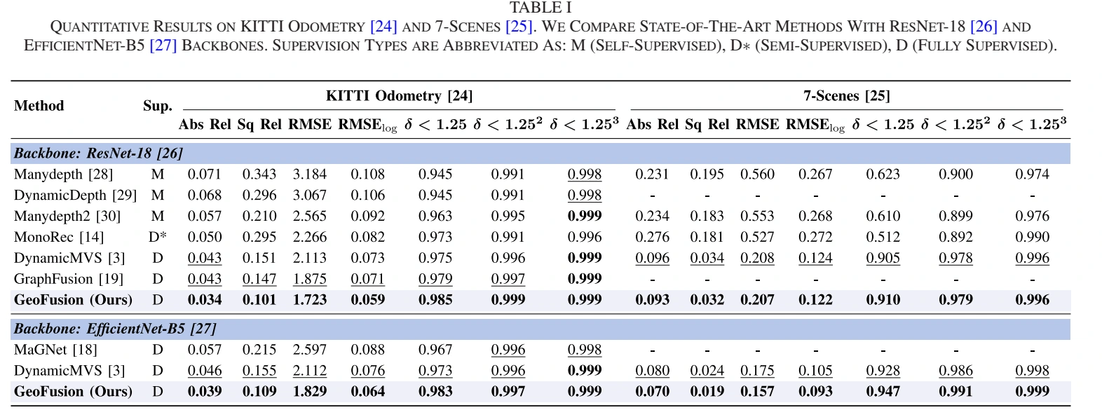
The main comparison covers outdoor KITTI Odometry and indoor 7-Scenes. With ResNet-18, GeoFusion reports KITTI Abs Rel of 0.034, compared with 0.043 for DynamicMVS, and 7-Scenes Abs Rel of 0.093, compared with 0.096. The paper also evaluates the larger EfficientNet-B5 backbone.
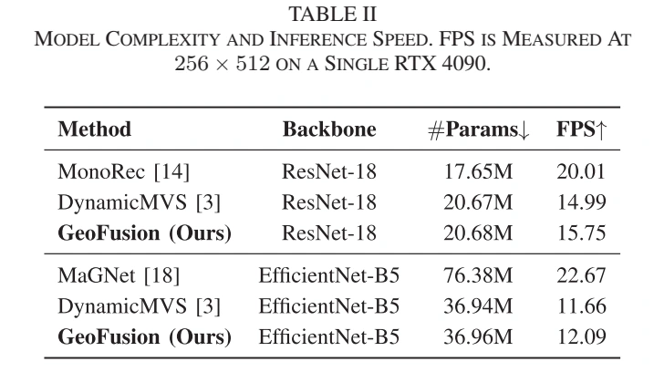
Table 2 reports the cost of the complete models, including parameter counts and speed at 256 × 512 on an RTX 4090. With ResNet-18, GeoFusion runs at 15.75 FPS versus DynamicMVS at 14.99 FPS, with both using 20.67 million parameters. These measurements belong to the stated hardware and input resolution.
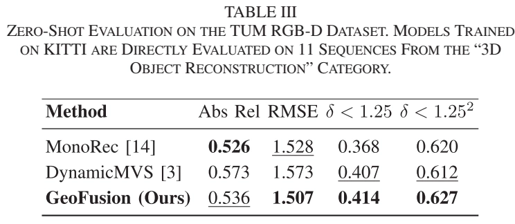
For zero-shot transfer, KITTI-trained models are evaluated directly on 11 TUM-RGBD reconstruction sequences. GeoFusion has the lowest RMSE in this comparison (1.507), while MonoRec has the lowest Abs Rel (0.526, versus GeoFusion’s 0.536). The table makes the metric-dependent comparison visible.
What the ablations test
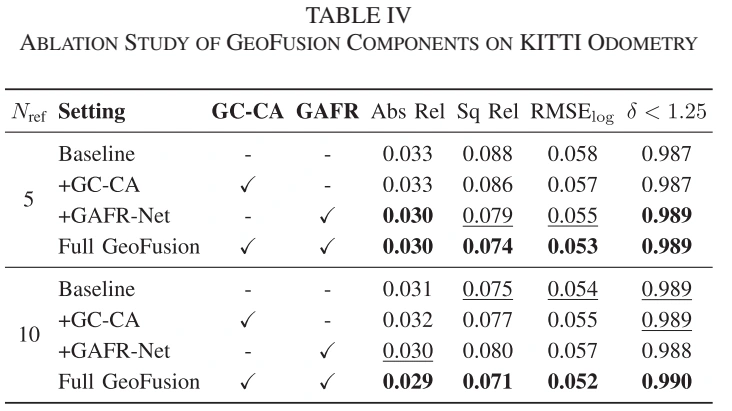
Table 4 separates cost aggregation from feature rectification at two reference-frame counts. Both contribute to the full model, and the combined configuration improves over either individual component.
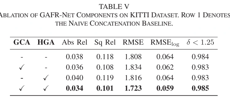
GCA and HGA have different roles. In Table 5, GCA alone improves Abs Rel from 0.038 to 0.036. HGA alone gives 0.040, while combining GCA and HGA gives 0.034. Global aggregation works best after the features have been geometrically rectified.
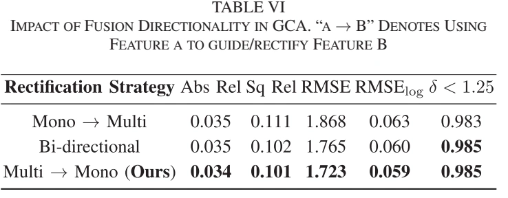
Table 6 directly tests fusion direction: multi-view-to-monocular rectification gives Abs Rel 0.034, versus 0.035 for bidirectional fusion and 0.035 for monocular-to-multi-view rectification. The same comparison also reports the remaining error and accuracy metrics.
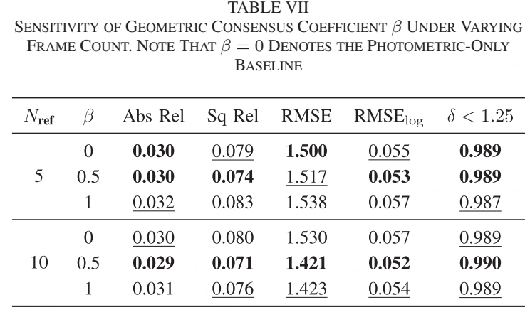
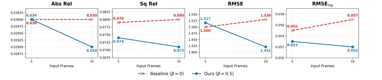
The sensitivity study varies the consensus coefficient and the number of reference frames. Without geometric consensus, adding views can also add inconsistent matching evidence. The selected coefficient β = 0.5 reduces error as the view count increases in the reported experiment.
Reconstruction and qualitative examples
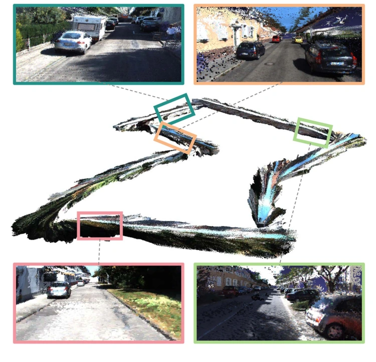
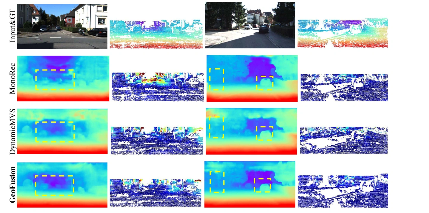
The reconstruction examples connect the predicted depth maps to recovered 3D structure. The comparison below pairs depth predictions with error maps; warmer colors indicate larger errors, and marked regions highlight fine structures and boundaries.