The problem
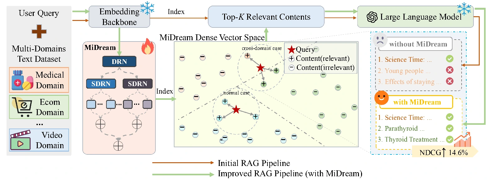
A single retrieval embedding model must often serve queries from very different domains. A shared representation can miss domain-specific vocabulary and distinctions, causing the retriever to select less useful documents for downstream generation.
How MiDream works
- A Domain Routing Network directs the query representation toward the appropriate domain.
- A Sub-Domain Routing Network selects two specialized gated linear unit experts within that domain, allowing finer adaptation without activating every expert.
- The embedding backbone remains frozen. Trainable experts transform its representations, so domain specialization does not require updating the entire embedding model.
Training follows three stages: pretrain the experts, train the domain router, then freeze that router while jointly training each domain-specific mixture of experts. Noisy gating and dropout encourage expert differentiation.
Hierarchical routing and representation adaptation
MiDream processes queries and document text with a pretrained embedding backbone, then adapts those vectors for retrieval. A Domain Routing Network (DRN) selects a domain-specific mixture. Within that mixture, a Sub-Domain Routing Network (SDRN) activates the top two gated linear unit experts and combines their transformed representations.
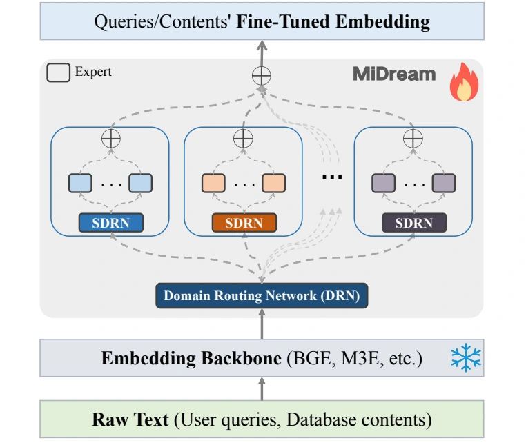
The first routing level addresses domain confusion, such as mixing medical and e-commerce queries. The second level gives each domain more than one expert transformation. The learned vectors can then be indexed and searched with standard dense-vector retrieval.
Why training is staged
- Expert pretraining: learn useful domain-specific vector transformations using contrastive retrieval training.
- Domain-router pretraining: train DRN to identify the domain of the input representation.
- Joint mixture training: freeze DRN and train the domain-specific mixtures, including their sub-domain routing.
The paper reports that unconstrained joint training can disrupt the domain gate. In the final stage, dropout and Expert-Augment Noisy Gating (EANG) encourage expert differentiation by perturbing routing logits and preventing identical experts from remaining interchangeable.
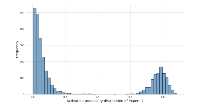
The expert-activation histogram shows specialization through unequal activation probabilities for different inputs, rather than a uniform allocation to every expert.
Retrieval setup and metrics
Experiments use the Multi-CPR e-commerce, medical, and video domains, with 10,000 training examples and 1,000 test examples per domain. Backbone comparisons include M3E and BGE. Adapted vectors are indexed with FAISS, and evaluation retrieves the top 10 documents.
F1 combines precision and recall. NDCG measures ranking quality, MRR emphasizes the rank of the first relevant document, and hit rate (HR) measures whether relevant evidence is retrieved. All four metrics are higher-is-better. The oracle comparison supplies the correct domain and is read as a domain-routing reference.
Across domains and within individual domains
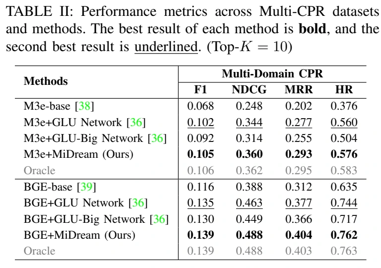
For BGE-based multi-domain retrieval, MiDream reports 0.488 NDCG and 0.404 MRR, compared with 0.449 and 0.366 for the equally sized GLU-Big model. With M3E, MiDream reports 0.360 NDCG and 0.293 MRR, compared with 0.314 and 0.255. The matched parameter counts help isolate the benefit of specialized routing from simply enlarging one transformation network.
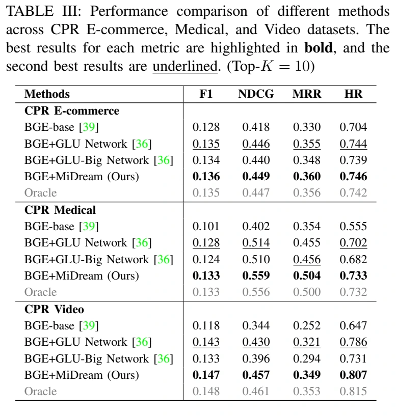
Domain-specific results show where the retrieval improvement occurs. In the medical domain, BGE + MiDream reaches 0.559 NDCG, versus 0.510 for GLU-Big. The full table also retains e-commerce and video results, including oracle comparisons.
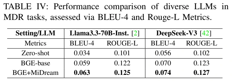
The paper additionally passes retrieved evidence to Llama-3.3-70B-Inst. and DeepSeek-V3. BLEU-4 and ROUGE-L compare downstream responses, connecting the retrieval experiment to the generation stage of RAG.
Routing, noisy gating, and computational cost
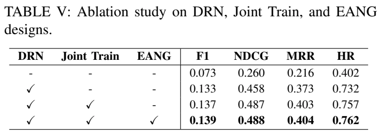
Removing domain routing gives NDCG 0.260 in this ablation. With DRN, it rises to 0.458; joint training reaches 0.487, and EANG reaches 0.488. The table reports the full set of metrics, so the marginal effect of each component remains visible.
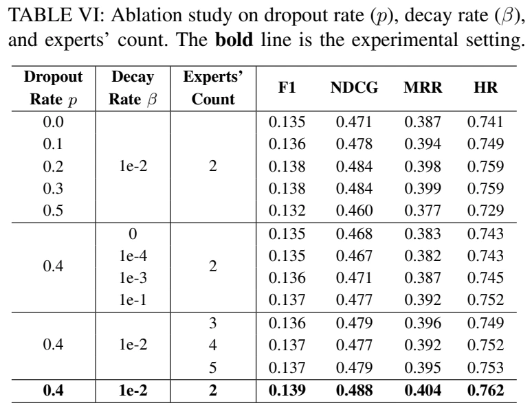
The sensitivity study varies dropout, auxiliary-loss decay, and the number of experts. The reported selected setting uses dropout 0.4, decay 0.01, and two experts.
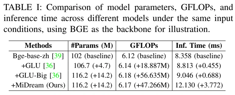
The efficiency table reports 116.2 million total parameters for both BGE + GLU-Big and BGE + MiDream. MiDream has slightly lower GFLOPs (6.17 versus 6.18) but higher measured latency (12.130 versus 9.046 ms). Lower arithmetic cost therefore does not imply lower end-to-end latency in this routed implementation.